This is part of a series of posts introducing the R language
Disclaimer: This text contains spoilers for one of the assignments for the Reproducible Research course at Coursera, if you plan on doing the Data Science specialization you might want to save this to read later or just read it now anyway, it’s just one of the many assignments :)
One of the very first things you’ll learn while working with data is that, many times, you will find that the dataset you have is missing information on important fields, the data dictionary (the piece that explains what each field is) is outdated or incomplete, the values available contain typos, duplication and many other inconsistencies that makes the data not ready for consumption. This data could have been generated by independent computer systems, could have been entered manually by humans or the data collection method might just have been ad hoc, bad data will be something you’ll deal with.
Cleaning and making sense of the data is indeed part of your work doing analysis, whenever you get a dataset, your very first step is to run some exploratory analysis to see what the values look like, find inconsistencies, missing data and perform basic cleanups before starting the actual analysis.
We’ll use the National Climatic Data Center Storms database as the example here. You can go through all files and merge them yourself (not recommended, as you will get newer files with a different format) or you can just download this condensed file with data from 1950 to 2011 about natural disasters that have happened in US territory.
Starting out
As with the previous article, I’d recommend you to use RStudio to follow through the steps we’ll be doing here. Let’s start by loading the file into a data frame:
zip <- bzfile("repdata-data-StormData.csv.bz2")
data <- read.csv(zip,
  strip.white=TRUE,
  colClasses=c("NULL","character","NULL","NULL","numeric","character",
  "character","character", "NULL",
  "NULL","NULL","character","NULL","NULL","NULL","NULL","NULL","NULL",
  "NULL","NULL","NULL","NULL","numeric","numeric","numeric","character",
  "numeric","character","NULL","NULL","NULL","NULL","NULL","NULL","NULL",
  "NULL","NULL"))
Given the file is large (if you unpack it it will be around half a GB) we don’t want to let R try to figure out the data types or load all columns, we will specifically select the columns we want to use and declare their types so the initial load is faster as R won’t be loading everything or trying to figure out what each field is.
Let’s look at the fields we have here:
names(data)
> [1] "BGN_DATE" "COUNTY" "COUNTYNAME" "STATE" "EVTYPE" "END_DATE"
> "FATALITIES" "INJURIES" "PROPDMG" "PROPDMGEXP" "CROPDMG" "CROPDMGEXP"
Most of the variables here should be self explanatory, let’s take a tour:
- BGN_DATE and END_DATE - the start and end of the event;
- COUNTY and COUNTYNAME - an unique identifier for the county and the name of the county;
- STATE - state of the county where the event happened;
- EVTYPE - this is the type of event that has happened, there are many types of events and they will require some clean up, we’ll get back to that in a bit;
- FATALITIES and INJURIES - the number of victims (either killed or injured) by the event;
- PROPDMG and CROPDMG - these are the cost of the damage caused by the event as property or crop damage;
- PROPDMGEXP and CROPDMGEXP - these are the multipliers to be applied to the crop and property damage values provided;
Cleaning up events
We’ll start by looking at the different types of events we have:
unique(data$EVTYPE)The unique function takes a vector and produces a new vector removing duplicates. This will print a list of 985 different types of events, but once you start looking around you’ll see different events as:
- “FLOOD/FLASH FLOODING”
- “FLASH FLOOD/FLOOD”
- “Flood”
- “THUNDERTSORM WIND”
- “THUNDESTORM WINDS”
- “THUNDERSTROM WINDS”
So we have typos, different casing and switched words all together for events that are supposed to be the same, we need a fix for that. While it would be great if I could tell you there is this magical R function that does this work for us, there isn’t. Due to the many different ways the same event is being presented differently here, the solution will be going through all the event names and changing them to a canonical one.
The first step is to make them all have the same casing and remove extraneous spaces from the beginning or the end of the event names, here’s how we can do it:
data$EVTYPE <- toupper(gsub("^\\s+|\\s+$", "", data$EVTYPE))Now we start to see the magic, we have a function gsub that takes a regex of what we should replace (the regex is mostly remove all spaces at the beginning or end of the text), the value that will replace (an empty string in this case) and lastly the vector (or string) where we will be replacing stuff.
Here we circle back to what we said in part 1 that everything in R is a vector, the gsub function works if we give it a single string or a vector of strings. Since even the single string is actually a vector of size 1, it doesn’t actually matter if it’s a single one or a collection of them, the function will happily apply the regex at every item and return a new vector (or a single item) with all items processed.
This is an example of vectorization, a very common pattern in R programs. While you would usually use a for/while loop in other languages to accomplish this result, in R most functions will accept a vector and apply it’s operation at every item in the vector automatically. It’s uncommon to see while/for loops in R programs, as most libraries will prefer to use vectorized functions to perform it’s work. Preferring vectorization will usually lead to better performance than trying to loop since libraries will try to optimize for this case.
Going back to our code, we then apply the toupper function to the vector that was produced by gsub which will now produce a new vector with all strings in upper case form.
We then assign the results of the computation to the data$EVTYPE field again, let’s check how many event types we still have:
length(unique(data$EVTYPE))
> [1] 890
This basic cleanup removed 95 duplicate event types, not perfect but still a great start for our job. The next step is, unfortunately, a manual operation, going through every event type and mapping it to a canonical version so we can have less noise when organizing this data. You won’t actually have to do this since I’ve done it already but whenever you find yourself in the same situation, find an expert in the field (which will probably be working with you anyway on the anaylsis) and remove the duplicates.
You should download the replacements.csv that contains the mappings from the original to the canonical event type. Once it’s downloaded and available to be used, load it at your R session:
replacements <- read.csv("replacements.csv", stringsAsFactors=FALSE)

eventFor <- function( evtype ) {
  replacements[replacements$event == evtype,]$actual
}
data$event <- sapply(data$EVTYPE, eventFor)
Running this will take a while since we have to produce results for 902297 rows, just be a little patient. Another option would be using a library like hash (yes, R does not have hashes natively) for faster access, but we can live with this waiting for now.
Going back to the code, we first read the replacements.csv file as usual but now we include the stringsAsFactors=FALSE option to prevent the code from loading everything as factors, which wouldn’t work for our case. By default, read.csv will assume all string fields should be read as factors, so make sure you either declare the types of every column as we have been doing or just disable factors if you don’t want them.
And now for something new, a function declaration!
As you can see, there isn’t much to say here, you declare a variable that will hold the function, use the function keyword, declare the parameters and then {} around the function body. You don’t need to include a return statement if the last line of your function returns the expected value (which happens here) and, perhaps the most interesting part of it, the function has access to all variables/functions declared at it’s external binding.
What does this mean?
It means that the use of replacements inside the function is perfectly valid since replacements is available at the environment where the function was defined. The functions you declare can use any variable declared out of them as long as they are visible when the function is declared. While this isn’t exactly a best practice if you’re coming from other programming languages, it simplifies our life for this case as this function will be called by someone else and not us directly. We know global variables are evil, but let’s can make a small exception here.
And now vectorization happens again. If you’ve been presented to functional languages before (or languages that have map and fold/reduce methods) you already know what sapply is doing. It calls eventFor for every value at data$EVTYPE and since eventFor produces a single value for every call, it merges them all into a new vector, effectively mapping every original value into a new one.
Again, this could be done by a for loop, but using a function like sapply is much simpler, given it also transforms the data into a vector so we can just merge it into our data frame. Which is also something that this code is doing, it is creating a new column, called event at the data frame to hold these new values.
length(unique(data$event))
> [1] 187
And now we only have 187 events to care about, progress!
Parsing dates
The cleanup work never stops, now we’re going to parse the dates:
data$date <- as.Date(data$BGN_DATE, "%m/%d/%Y")
data$year <- as.POSIXlt(data$date)$year+1900
This gives us dates with actual fields (instead of just a string) and the year in separate as we’ll be using it later for other comparisons. Just like the events case, we save them as new columns at the data frame, this allows us to circle back to the original columns and re-process them if necessary. You should avoid overwriting the original fields at your data frames as you might have to re-process the original data later.
Assessing damage
We now consider the damage costs caused by the events. The original data dictionary for this dataset said the multipliers PROPDMGEXP and CROPDMGEXP could assume the values K (for thousands), M (for millions) and B (for billions) of USD. Let’s look at what the actual values at the dataset look like:
unique(data$PROPDMGEXP)
> [1] "K" "M" ""  "B" "m" "+" "0" "5" "6" "?" "4" "2" "3" "h" "7" "H" "-" "1" "8"
unique(data$CROPDMGEXP)
> [1] ""  "M" "K" "m" "B" "?" "0" "k" "2"
Not exactly what we were expecting, right?
Time for another transformation, now with the multipliers.csv file. Here’s the code to load and use it:
data$PROPDMGEXP <- toupper(data$PROPDMGEXP)
data$CROPDMGEXP <- toupper(data$CROPDMGEXP)

multipliers <- read.csv("multipliers.csv", colClasses=c("character", "numeric"))

mapDamage <- function(damage, mapping) {
  damage * multipliers[multipliers$key == mapping,]$number
}
data$property_damage <- mapply(mapDamage, data$PROPDMG, data$PROPDMGEXP)
data$crop_damage <- mapply(mapDamage, data$CROPDMG, data$CROPDMGEXP)
data$total_damage <- data$property_damage + data$crop_damage
Here we’re doing mostly the same of what we did with events, the main difference is that now we’re using mapply instead of sapply to calculate the results. Why is that?
sapply expects to call the given function with a single argument, but to actually perform the calculation here we need both the damage value and the multiplier for that value, so we need to give our functions the pair of damage and multiplier values. mapply comes to the rescue here since it allows us to provide N vectors and it is going to call our function with every sequence of the N values, which in our case is every damage and it’s own multiplier.
Again, no loops are necessary anywhere since all operations are vectorized. At the end we also sum the damage values to calculate the total damage for every event. Since R knows we’re dealing with vectors here it knows what we want is to sum every row and not the whole vectors, so what is happening at that last line is that every row will have it’s property and crop damage summed and included at a new column.
split-apply-combine
This natural disasters database has been collected from various different sources since the 50’, so it might be nice for us to look at how the data collected for every year changes. Our question here will be, how many different events happened on every year so far?
Aggregating values based on categorical variables (which would be our year here) is such a common task on data analysis that it has it’s own name, the split-apply-combine pattern. It’s called like this because you first split the data based on a specific column, then you apply a function to every subset of the data and at the end you combine all the different results into a single data set.
Let’s see how we could build our events per year dataset now:
years <- split(data, data$year)
events_per_year <- lapply(years, function (x) length(unique(x$event)) )
result <- do.call(rbind, events_per_year)
result here is a matrix with the following values:
1950    1
1951    1
1952    1
1953    1
1954    1
1955    3
1956    3
1957    3
1958    3
1959    3
1960    3
1961    3
1962    3
1963    3
1964    3
1965    3
1966    3
1967    3
1968    3
1969    3
1970    3
1971    3
1972    3
1973    3
1974    3
1975    3
1976    3
1977    3
1978    3
1979    3
1980    3
1981    3
1982    3
1983    3
1984    3
1985    3
1986    3
1987    3
1988    3
1989    3
1990    3
1991    3
1992    3
1993   59
1994   67
1995   98
1996   77
1997   78
1998   70
1999   74
2000   65
2001   77
2002   65
2003   43
2004   37
2005   41
2006   43
2007   44
2008   44
2009   44
2010   44
2011   44
As you can see, before 1993, very few different events were recorded every year, not because they did not happen, but because the rules to track these natural disasters were different. These discrepancies are going to be all over the place as you work with data and you should always consider what it will mean for your end results, as making direct comparisons between the years before 93 with the ones that come after it will surely generate different results. In this case, we’re better off using either one or the other side of the data set and not everything.
As for the code, the split function takes the data set as the first parameter and the categories as the second. You don’t have to provide unique values here, split is smart enough to figure out what you mean and correctly split the values on every unique option. This produces a list of year -> dataset subset for that year.
Then we use the lapply function at this list, it calls the function you give it for every item at the list and since for our case every item in the list is the subset for a specific year, all we have to do is to select the unique event types and calculate the length of the produced uniques. See how we declared the function right at the parameter? That is an anonymous function, really useful when you want to provide a one-line function to xapply methods.
And at the end we use the do.call function to call rbind on every item of our lists so we can turn them into a matrix. It’s as if we called rbind providing the year and the value on every call, do.call removes the need of manually looping to do it.
And while this is all good pure R standard library programming, you don’t actually want to do this tedious work whenever you need to run an split-apply-combine operation, the plyr library comes with all this baked right inside of it so you don’t waste your time doing it.
First, let’s install it:
install.packages("plyr")Once the installer is finished, here’s all the code we need:
require(plyr)
events_per_year <- ddply(
  data,
  c("year"),
  summarise,
  count=length(unique(event))
  )
The plyr package contains various methods that do the split-apply-combine scenario on many different kinds of inputs producing different outputs. The ddply method is one that takes a data frame and produces a data frame (that’s why it’s dd), but you could use a method that produces a list or any of the other methods available at the library.
Here we provide our data frame as the first argument, then the list of variables we want to use as the split, then how the result will be built (summarise means we want a new object to be built from scratch) and then the fields we will want included at this new data frame. For this case, all we want is the count field, the value for the field is the operation you want to apply (it does not have to be a function) and it has access to all fields at the data frame you provided, that’s why we just say event here instead of data$event.
The result of this function is a data frame with year and count fields, the same we had above with our manual operation. So, whenever you’re going to play around with these split-apply-combine operations, use plyr and be happy!
Playing around with the data and basic plotting
Given we know the information before 1993 is much different than the one available after it, let’s start by creating a subset of the data that contains events starting at 1993:
filteredData <- data[data$year >= 1993,]This is known in R parlance as subsetting since you are creating a subset of the data based on some conditional. If you run data$year >= 1993 alone the result will be a logical vector containing one value for every row inside data with either TRUE (if the row matches the condition) or FALSE (if it does not) and when you use this vector as the row part for the [] operator every row that matches a TRUE value will be returned. You can use boolean operators like & and | when performing these comparisons as well for compound matches just like any other programming language.
Let’s group injuries and deaths per event:
healthConsequences <- ddply(
  filteredData,
  c("event"),
  summarise,
  total_deaths=sum(FATALITIES),
  total_injuries=sum(INJURIES)
  )
This gives us the full list of events and their casualty numbers. Now let’s sort this data frame per fatalities:
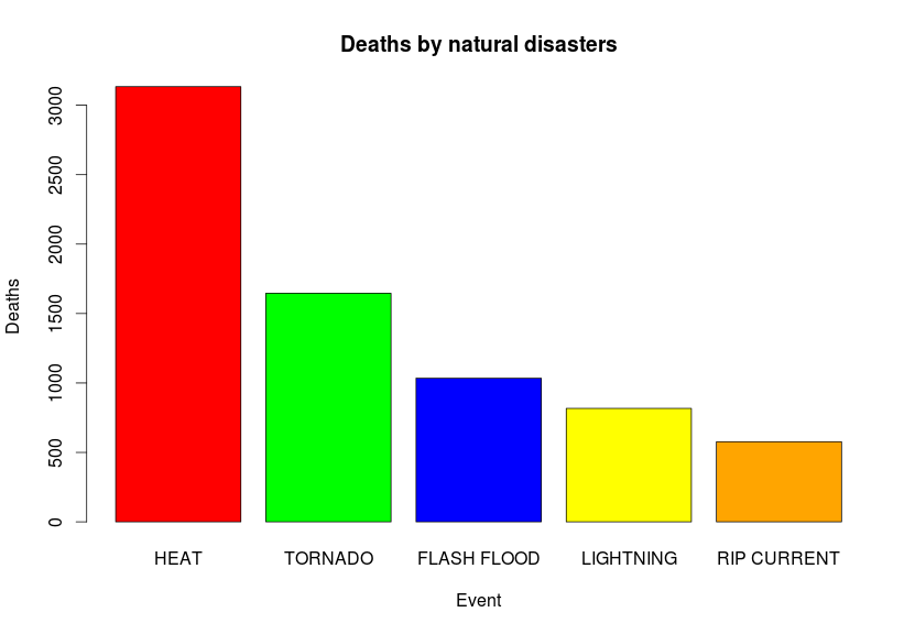
mostDeadly <- healthConsequences[order(-healthConsequences$total_deaths),]Now we have a data frame of the most deadly events so far sorted in descending order. Let’s plot the numbers for the top 5 events:
barplot(
  mostDeadly[1:5,2],
  names.arg=mostDeadly[1:5,1],
  col=c("red", "green", "blue", "yellow", "orange"),
  main="Deaths by natural disasters",
  xlab="Event",
  ylab="Deaths")
Since we have one categorical and one numeric variable to use, the most direct option for a plot is a barplot, we grab the top 5 rows and print them. The code itself is self explanatory, first we provide the numeric values, then we set the names.arg to be the top 5 field names, we provide color names for the bars, titles and legends for the generated plot.
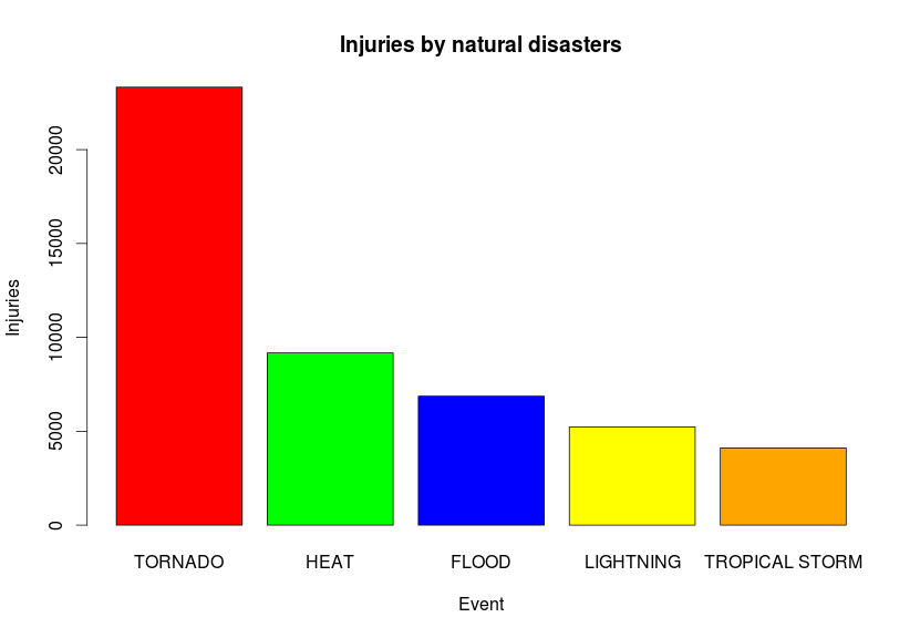
We can also do the same for the most injuries:
mostInjuries <- healthConsequences[order(-healthConsequences$total_injuries),]Let’s look at the top 10 values:
               event total_deaths total_injuries
166          TORNADO         1646          23328
78              HEAT         3134           9176
60             FLOOD          508           6870
110        LIGHTNING          817           5232
168   TROPICAL STORM          313           4113
164     THUNDERSTORM          201           2452
97         ICE STORM           89           1977
59       FLASH FLOOD         1035           1800
185 WILD/FOREST FIRE           90           1606
93         HIGH WIND          293           1471
And if we plot them to compare:
barplot(
  mostInjuries[1:5,3],
  names.arg=mostInjuries[1:5,1],
  col=c("red", "green", "blue", "yellow", "orange"),
  main="Injuries by natural disasters",
  xlab="Event",
  ylab="Injuries")
We’ll get:
Now start playing around with the damage data to figure out which is the most expensive type of disaster that has happened over these years, there’s a lot of interesting information you can figure out from this simple dataset.
Patience and exploration are key
The data you’ll find out there is unlikely to be clean and clearly defined, you should be able to explore it, find it’s weak points, find it’s missing details and then start your analysis. Ignoring that the data you have might be misleading is a sure path to bad and unreliable analysis and you don’t want to do be doing that, do you?